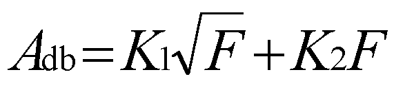
In graphical form:
Back to home
Modified 10/12/2001
In December 1993, the New Ham Companion section of QST carried an article
written by ARRL staff writer, Steve Ford, titled, "The Lure of the Ladder
Line." While I am far from a "new ham", for several years I taught beginning
ham radio courses at the local community college, so I take a special interest
in things directed to beginners. I believe it is imperative that beginners
should not be misled, as bad advice is just like a bad habit; it is hard
to overcome.
After reading the article I had several concerns that I decided to share
with the editors. I wrote a letter to Paul Pagel, the editor of QST's
"Technical Correspondence" column, in which I expressed my opinion that
while most of the information was good; I felt that some points were
missing. While my letter was never published, it did start a series
of letters between the ARRL Antenna Book editor, Dean Straw, and me.
One of the things that I thought was lacking in the article was the absence
of any concern
for tuner and balun losses. At the time this correspondence was taking
place I had access to EESOF Touchstone, a professional grade RF CAD program. I
did a number of "what-if" scenarios involving typical transmatch circuits
and the possible losses therein. I wrote a
letter to Dean in which I
spelled out some of my findings.
Not long after, in QST for January 1995, Andrew Griffith, W4ULD,
wrote a paper titled, "Getting the Most Out of Your T-Network Tuner,"
which presented some of the points that I had raised earlier. Then the
April and May 1995 issues of QST carried a two-part paper by Frank Witt,
AI1H, titled, "How to Evaluate Your Antenna Tuner." Witt showed data
taken on popular tuners while matching various standing wave ratios.
In most cases, the mismatched loads were resistive (reactive loads can
behave even worse). In one instance the observed tuner loss exceeded 75%
(6 dB), with what I assume was optimum adjustment.
In a later letter Dean invited me to write something for the Fourth
Edition of the ARRL Antenna Compendium but the deadline was too close for me
to respond. Work and other issues prevented further thought about the
subject until the call for papers for the Sixth Edition of the ARRL
Antenna Compendium was received. I asked Dean whether he would still
be interested and he said yes. This manuscript for
"Balanced
Transmission
Lines in Current Amateur Practice" was my submission.
(Published with permission of ARRL)
The Mathcad file of Appendix B can be downloaded by right clicking
here
and selecting "save link as."
After receiving a request from Press Jones (The Wireman) for permission to use
data from my Compendium paper and his question about whether I could extend
the data to lower frequencies, I decided to revisit the subject.
I discussed the basic measurement process in Appendix A. Error correction and
network analysis. In the last paragraph of the appendix, I stated that the
calibration process can remove the effects of the cable between the instrument
ports and the line under test. This is true to a point; however, the additional
loss in the extension cables does degrade accuracy to some extent. In addition,
when performing the through calibration, the business ends of cables were
connected together, and then for the measurement were separated to reach
the ends of the 12 foot long line under test. The movement and flexing of
these cables can affect the calibration somewhat, particularly the phase portion.
I also stated that the major accuracy limitation is the uncertainty of the
reference standards. This is a result of the fact that I was performing
calibration at the balanced end of the baluns. The physical realities were
that as the coax exited the balun, the leads were pigtailed out, and in an
effort to maintain some degree of consistency, they were tied to some posts
riveted into a piece of bare G10 board material.
The standard (50 Ohm) load used
for calibration was the precision 3.5 mm (beadless SMA) male coaxial load from
the HP calibration kit. Therefore, I was calibrating a "balanced"
test port with an unbalanced load, however if the baluns are doing their job,
and there is no ground connection, (there wasn't) the instrument shouldn't
be able to tell the difference.
Because I wasn't about to solder one of the standards out
of $3000 calibration kit into my circuit, I installed a 3.5 mm female
connector across each set of terminals and left them in place for the duration.
These connectors and the terminal posts added some unavoidable fringing
capacitance to the "open" circuit.
The "short" calibration is similarly
flawed, as the short was actually about 0.75 inches long. This was the
distance between the terminals and was dictated by the spacing of the ladder
line conductors. A wire 0.75" long is not a short at 150 MHz.
In retrospect I wish I had a better handle on the
performance of the baluns. Characterizing these would have been another
project. Any loss in the baluns (there shouldn't have been any) was calibrated
out; however, less than perfect balance gives rise to common-mode current in
the line under test. This in turn can cause some line radiation and increase
the apparent loss of the transmission line. After completing my work I
discovered a paper,
"Characterization of Balanced Transmission Line by
Microwave Technique", IEEE Transactions on Microwave Theory and Techniques,
Vol. 46, No. 12, December 1998
(download zip) that discusses this. This radiation loss,
if any, is not easily accounted for in the simulations, as it is neither
conductor loss nor dielectric loss.
In the original paper, I presented data that had been derived from the raw
measured data using ARRL Radio Designer (ARD) software. ARD has two transmission
line models, one a so-called balanced line and the other a coax cable model.
Initially, since I was working with balanced line, I restricted the analysis
to the balanced line model. One problem with this model is the fact that it
has only one loss coefficient, i.e. X dB/unit length. I have no idea about
how this coefficient is determined and how it accounts for both wire (skin
effect) loss and dielectric loss.
As I stated in the paper, I let ARD's optimizer attempt to make the response
of the ideal model equal the response of the measured data. It was the result
of this optimization that I presented in the paper. Since that time, and after
posting the paper here, I heard from Dan Maguire, AC6LA, who has built a
very nice Excel spreadsheet for
doing transmission line calculations. He
asked whether I would be willing to pass along some of the measured data
to him, which I gladly did.
Dan used Excel's solver and the standard transmission line equations to derive
the same data that ARD did, with the exception that he solved for the loss
coefficients separately. These are K1, the loss due to wire conductivity
(proportional to the square root of freq) and K2, the loss due to the
dielectric (proportional
to freq). Both of these are in dB/unit length, usually dB/100 feet/MHz.
Our data correlated remarkably well using the "dry" data, however, it was
somewhat different using the "wet" data. (As an aside, I regret including
so much about the wet condition. I tried to make it clear that this was
really worst case and not something that would be seen in practice, but there
has been so much negative commentary about it, that it detracts from the point
I was trying to make.)
When Dan solved for the loss in the wet condition, he rightly assumed that
the conductor loss would remain the same and just solved for the dielectric
loss. Because of the divergence of our two solutions, I suspected that ARD's
simpler model was inappropriate when dielectric losses were out of the ordinary.
Since the time I did the original work, Ansoft has released their student
(free) version of their
Serenade SV
r-f CAD program. I used Serenade to perform similar analysis as before,
only this time I used the
coax model that has the two separate loss coefficients. The optimizer routines
in Serenade seem to be more robust and there are more options for seeking
convergence.
What I found using the different optimization routines was interesting, or
upsetting depending on your point of view. In the ideal case, it should not
matter how the optimizer works, as the model should converge to match exactly
the measured data. Alas, because of some of the issues raised above concerning
the less that ideal measurement and calibration process, the measured data does
not represent an "ideal" transmission line. Furthermore, upon reflection
(no pun intended) I don't believe that window line is in the strictest
sense a "pure" transmission line.
The impedance of the line changes slightly at the beginning and end of each
"window." In Chapter 3 of General Radio's publication, Handbook
of Coaxial Microwave Measurements it is said, "Because each step
causes fringing of the
fields, predominately the electric field, there is an effect that is
approximated by a small capacitive reactance at each discontinuity."
I don't begin to know whether this is of significance when the line is
operating at relatively low frequency, but I do believe that as the frequency
increases, the effect might become bothersome. I also suspect, but cannot
prove, that these discontinuities exacerbate the poor performance seen when
the line is wet.
What I saw in the modeling was that depending on the optimization method used,
I got different answers, primarily for the dielectric loss coefficient.
I believe this results from the different weights placed on matching each of
the measured s-parameters by the different routines. Because of the calibration
issues raised earlier, the uncertainty in the balun and attendant possibility
of excess line radiation and maybe the fringing effects, I believe that the
measured data are "corrupt" to some (undetermined) degree. As a practical
matter, I doubt that any of this is significant, however, if I say that the
loss of a line is 0.4 dB/100 ft now, and before, I said it was 0.3 dB, someone
is going to complain and say that I don't know what I'm talking about.
In the model, there are four line parameters that are variable: Characteristic
impedance (Zo), propagation velocity (Vp), conductor loss coefficient (K1) and
dielectric loss coefficient (K2). Zo and Vp converged very quickly to stable
values. After they did, I fixed them at those values and then performed further
optimization, looking for a better fit for the two loss coefficients.
Using the "random" search method, the resulting coefficients showed that
there was almost no dielectric loss contribution and the line attenuation
was primarily dependent on the conductor loss. The slope of the attenuation
curve was predominately a function of the square root of frequency.
Using the Levenberg-Marquardt search method, which has different error
functions, the coefficients leaned toward attenuation more dominated by
dielectric loss. The effect of these differences is that at the lower
frequencies there isn't much difference but as the frequency increases,
the slope of the attenuation curve increases when the dielectric coefficient
begins to dominate.
I saw a little bit if this same slope change for the "true" open wire control
sample, that has essentially no dielectric, so I suspicion that there is some
line radiation going on, above what theory says there should be. Also the
effect of calibration errors will be more significant at the higher test
frequencies so all of this compounds to confuse the modeling process.
Nevertheless, the slope is greater when there is dielectric present, so
I cannot attribute all of the effect to radiation and calibration error.
A lot of this comes down to picking flyspecks out of the pepper. So,
what I have done is an "engineering approximation" (known in some circles
as a wild-ass guess) and averaged the results.
The results are consistent in that the loss with solid wire is lower than
the same size stranded wire, and larger wire has lower loss than smaller
wire. For the same sized wire, less dielectric is better.
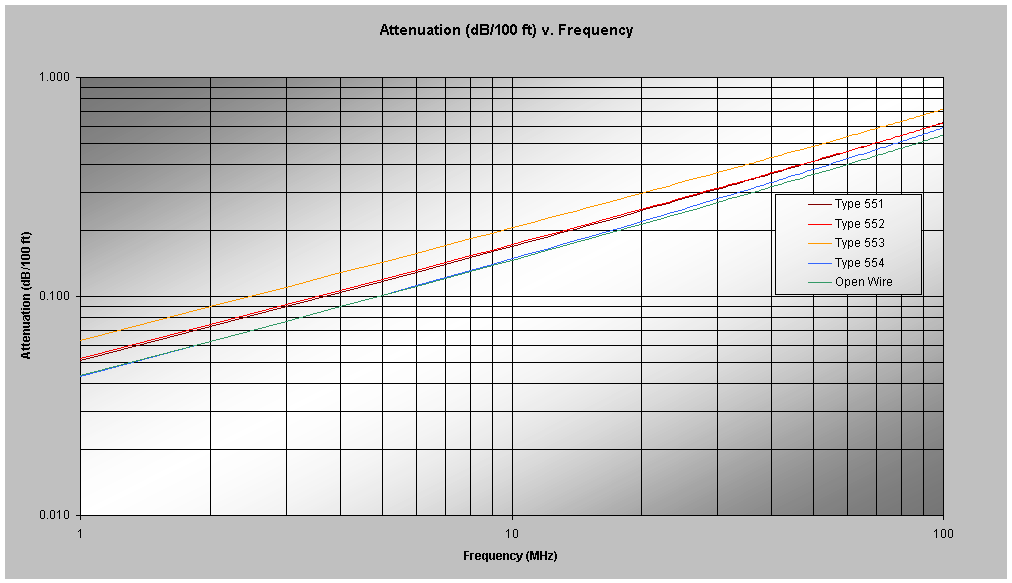
The revised numbers are as follows:
| Type No. | Nominal Impedance (Ohm) | Effective Dielectric Constant | Propagation Velocity | K1 | K2 |
| 551 | 400 | 1.23 | 90.2% | .0496 | .0012 |
| 552 | 370 | 1.19 | 91.7% | .0510 | .0010 |
| 553 | 390 | 1.24 | 89.8% | .0621 | .0009 |
| 554 | 360 | 1.16 | 92.8% | .0414 | .0017 |
The
line attenuation in dB/100 feet at any frequency can be found by:
Back to home
In graphical form:
Modified 10/12/2001